Command-line Examples

For the most basic usage of rNets through its command-line interface we recommend checking first the Basic Usage. In this section, more more comprehensive examples covering more detailed graph customization will be included.

My first reaction graph

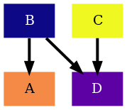
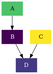
To introduce the minimal components of rNets we will create a very simple reaction network, which is shown below:

First we will start writing the Reactions file and then we will write the Compounds file. In this case we have 2 reactions, A -> B and B + C -> D. To create our csv we will start with the following table, which we can create in your preferred spreadsheet editor:

cleft	cleft	direction	cright	energy	name

The details of each column are explained in the File Formats but the key thing here is that we have one reaction that has 2 reactants but no reaction leading to the formation of 2 products we will only need one cright (Compound at the RIGHT side of the reaction) column.

Now we can proceed to add the first reaction:

cleft	cleft	direction	cright	energy	name
A		->	B	1.0	R1

If we were to save the file with our editor as a csv it would look like:

cleft,cleft,direction,cright,energy,name
A,,->,B,1.0,R1

Note

We are currently adding an energy of 1.0eV. This value is not important for getting the reaction network right, but will impact the coloring and thickness of the arrows in the next examples.

Now we add the second reaction:

cleft	cleft	direction	cright	energy	name
A		->	B	1.0	R1
B	C	->	D	1.0	R2

which we will save as the file reactions.csv.

cleft,cleft,direction,cright,energy,name
A,,->,B,1.0,R1
B,C,->,D,1.0,R2

Note

Please notice how the second cleft column has been left empty for the first reaction. If the second reaction did not involve a second reactant we could have completely removed the column, or left it with empty spaces and in both cases rNets will properly treat the reactions as unimolecular reactions.

Now that we know all species involved in the reactions we can write the Compounds file which. As it is also a csv file we will again use our spreadsheet editor for generating the table:

name	energy
A	0.0
B	0.0
C	0.0
D	0.0

When we save the table as the csv file compounds.csv it will look like:

name,energy
A,0.0
B,0.0
C,0.0
D,0.0

Note

Again, for this example we will use the value of 0.0eV for the energies energy without paying much attention to it, as we are only interested in generating an initial graph.

Now that we have created both of our input files, the last two steps are to generate the dot file and the image file, these steps are exactly as it is shown in the Basic Usage.

$ python -m rnets -cf compounds.csv -rf reactions.csv -o reaction_network.dot
$ dot -Tpng reaction_network.dot -o reaction_network.png

If we want an editable image we recommend doing the final conversion to an svg instead of a png:

$ dot -Tsvg reaction_network.dot -o reaction_network.svg

Drawing a thermodynamic graph

For rNets, the absence of information about concentrations in the compounds.csv will always lead to an energy-based representation. So the only difference with My first reaction graph example is that this time we will be providing different energy values. Let's assume that we updated the energies of the previous tables to generate the reactions.csv and compounds.csv files respectively

cleft,cleft,direction,cright,energy,name
A,,->,B,4.0,R1
B,C,->,D,7.0,R2

name,energy
A,0.0
B,1.0
C,0.0
D,-2.0

After updating the energy values of reactions.csv and compounds.csv we can proceed with the generation of the graph.

$ python -m rnets -cf compounds.csv -rf reactions.csv -o reaction_network.dot
$ dot -Tpng reaction_network.dot -o reaction_network.png

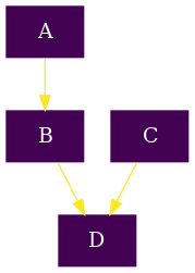
The resulting graph will look like:

If we compare it with the graph generated in My first reaction graph example we can now observe how, with the default color scheme, the most stable compounds are colored in a darker color ( D ) while the least stable compounds ( B ) are in a lighter color. Also we can observe how the reaction with the lowest barrier has a thicker and darker color than the other reaction.

Drawing a kinetic graph

As indicated in the previous section, the absence of information about concentrations in the compounds.csv will lead to an energy-based representation. So, in order to change to a concentration-based representation we need to first update our compounds.csv which we can do directly on the file or using a spreadsheet editor.

name	energy	conc
A	0.0	0.75
B	1.0	0.1
C	0.0	1.0
D	-2.0	0.25

After adding the concentration column and saving our file as a .csv it will look like this:

name,energy,conc
A,0.0,0.75
B,1.0,0.1
C,0.0,1.0
D,-2.0,0.25

The reactions.csv file instead, requires no further change, so we will borrow it from the Drawing a thermodynamic graph example:

cleft,cleft,direction,cright,energy,name
A,,->,B,4.0,R1
B,C,->,D,7.0,R2

After updating our compounds.csv and with the already prepared reactions.csv we can proceed with the generation of the graph.

$ python -m rnets -cf compounds.csv -rf reactions.csv -o reaction_network.dot
$ dot -Tpng reaction_network.dot -o reaction_network.png

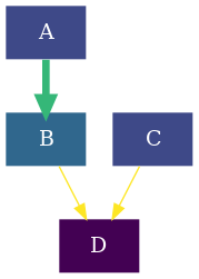
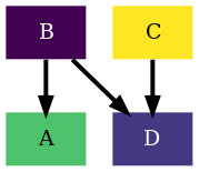
The resulting graph will look like:

Compared with the previous two examples we can observe clear differences. Same as the Drawing a thermodynamic graph example, the colors of the different in this case are light for compounds in high concentration, while dark colors corresponds to low concentration species. The major difference with the previous two examples is in the arrows. The arrows here represent the net reaction rate, a thicker arrow means a larger net rate and a thinner one a lower net rate. The direction of the arrow shows which species are being mainly generated and which ones are being mainly consumed. This feature is specially interesting when dealing with complex reaction networks where the concentration effects are difficult to predict, as it provides a visual cue.

Using different energy units

In this example we will get introduced to the chemical configuration class ( rnets.chemistry.ChemCfg ). to illustrate its usage we will borrow the Drawing a kinetic graph example.

First, we are going to rewrite our compounds.csv and reactions.csv in kcal/mol which we can easily do in our preferred spreadsheet editor.

name	energy	conc	energy(eV)
A	0.0	0.75	0.0
B	23.1	0.1	1.0
C	0.0	1.0	0.0
D	-46.1	0.25	-2.0

We remove the energy(eV) column and save the file as a csv

name,energy,conc
A,0.0,0.75
B,23.1,0.1
C,0.0,1.0
D,-46.1,0.25

We proceed similarly with the reactions.csv obtaining the file:

cleft,cleft,direction,cright,energy,name
A,,->,B,92.2,R1
B,C,->,D,161.4,R2

The next, we proceed to generate the .dot file as we did in the previous examples. However, this time we need to specify the energy units within the command:

$ python -m rnets -cf compounds.csv -rf reactions.csv -o reaction_network.dot --units kcal/mol
$ dot -Tpng reaction_network.dot -o reaction_network.png

If the energies provided were at a reference state of 500K we would need to specify also the temperature in the command line:

$ python -m rnets -cf compounds.csv -rf reactions.csv -o reaction_network.dot --units kcal/mol --temperature 500

Formatting our graph

In this final example we will cover how to change the basic formatting of the graph. The options that we can change are listed in the command line help Command-line help although an advanced configuration can be done using the Graph, Node and Edge OPT in this example we will focus on the less advanced options as they requrie no knowledge of the details of graphviz. We will use the following compounds.csv

name,energy,conc
A,0.0,0.75
B,1.0,0.1
C,0.0,1.0
D,-2.0,0.25

and the following reactions.csv

cleft,cleft,direction,cright,energy,name
A,,->,B,4.0,R1
B,C,->,D,7.0,R2

We are borrowing these files from the Drawing a kinetic graph example. As in the Using different energy units example all we will need to is to specify the flags in the command line. Lets assume that we want two different changes, the first one being the colorscheme and the second one the edge width. In other words, we want the edges to be thicker and we will use a different color palette.

First, lets address the edge width. The default value is 1, so we will make it 3. to specify this change we will need to add to the command line the flag --width 3. Consecuently the command line will look like:

$ python -m rnets -cf compounds.csv -rf reactions.csv -o reaction_network.dot --width 3

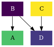
And now we generate the .png file

$ dot -Tpng reaction_network.dot -o reaction_network.png

Next, to change the colorscheme we will use one of the predefined ones which are magma, plasma, inferno, viridis and cividis . Specifically, the viridis is the default value, so we will use the plasma . As we did with the edge width, we will need to include the flag --colorscheme plasma .

$ python -m rnets -cf compounds.csv -rf reactions.csv -o reaction_network.dot --width 3 --colorscheme plasma

And now we generate the .png file

$ dot -Tpng reaction_network.dot -o reaction_network.png